Listening Position Measurements

Measurements at the listening position are nice to achieve a quick „objective“ sound quality documentation of an audio system. Let’s have a look at the basics.

John Atkinson of Stereophile magazine keeps a certain procedure of such measurements for long time now, enabling comparisons. Issue may 2019 page 73, a wilson audio speaker report: „I average 20 1/6-octave-smoothed spectra, taken for the speaker placed first in the left and then in the right positions using a 96 kHz sample rate, in a vertical rectangular grid 36 inch wide by 18 inch high and centered on the positions of my ears.“

The System

To show some measurements and the effect of smoothing and averaging I use the same speaker (Topo, one of my regular models) as before.
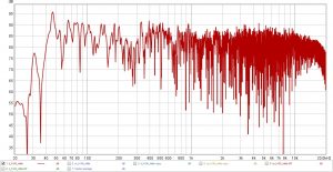
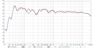
The picture on top shows raw versa 1/6 octave smoothed data for left and right speaker, at the listening position. Listening position is 180 cm in front of the speakers. Low frequency room modes show up similar to measurements in previous blogs. Most significantly a boost at 46 Hz and a cut below.

All measurements done with REW (Room EQ Wizard) using miniDSP UMIK-1 (cheap USB microphone that works perfectly with REW). REW is free, and gets better every year – very nice, and easy to use.

The Procedure

I took multiple measurements at and around the listening position. Starting point is my nose while listening. 25 cm to the right and left, and 20 cm behind the same three positions again. The whole thing repeated at two other heights, 10 cm up and down starting at a height of 100 cm.

Primary results are raw (no smoothing) 500 ms windowed data. In my top picture you can see the heavy room influence (comb filtering of left and right loudspeaker signal), that completely hides the anechoic speaker response at higher frequencies. And the result of 1/6 octave wide smoothing.

The Power of Smoothing

What can we do with a single measurement at the listening position to retrieve information about the HF balance of the sound? It is impossible to interpret the raw data, look at the unsmoothed left speaker response:

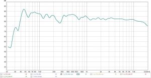
Our hearing adapts to room acoustics. It is used to identify the timbre of sound sources in different rooms, suppressing the influence of room reflexions. It „ignores“ the strong high frequency ripples of the raw response curves. Therefore, to make meaningful measurements, smoothing seems reasonable. While that characteristic of our hearing is frequency dependent, it is similar to the 1/6 octave smoothing. 1/6 octave smoothed left speaker response shown here:

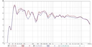
The following graph compares 1/6 to 1/24 octave wide smoothing of the left speaker data:

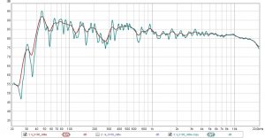
The 1/6 octave smoothing hides a lot of room mode information. Therefore, we could use a narrower 1/24 octave smoothing to still show meaningful HF information and keep the sharper LF ripples.

Spatial Averaging

Instead of averaging in the frequency domain, we can spatially average sets of different microphone positions. Each position contains different sound paths, hence different comb filtering. If we sample enough positions around our listening position, averaging them into one response curve should work similar to spectral smoothing. But might be more „realistic, since our left ear hears both speakers on a different location to the right one. And we hardly sit et exactly the same „sweet spot“ all the time.

Let us look at the result of averaging 18 positions proceeded according to above description, without smoothing the result. Left loudspeaker shown:

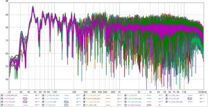
The violet result is much smoother than the raw curves, but not as smooth as 1/6 octave frequency smoothing.

Watch the Scales

If you look at measurements in magazines and advertisings, always look at the vertical scale first: A very smooth response curve may not only be the result of wide-band smoothing. It is easily achieved by compressing the vertical range.

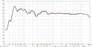
For example let us compare right and left loudspeaker response to determine the symmetry of our stereo setup. We compare 1/6 octave smoothed responses with resolution as above:

And zoom in a bit, vertically:

Easier to read, isn’t it?

How about doing the opposite, to achieve „impressive“ results?
First, we combine left and right spatially averaged and 1/6 octave smoothed curves as described in the procedure section.

Using the result, we increase the vertical range a bit:

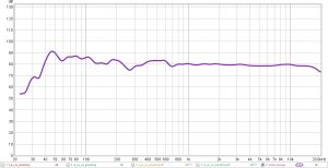
Looks nicer, right? There are still some websites showing 10 dB / diversity plots!
So, to compare different sources of data, always watch the scales, and look for information about the measurement procedure.