
Measuring Loudspeakers – intro
For me as a loudspeaker designer and acoustician measuring loudspeakers is mostly about the far field pressure response (magnitude and phase).
With such measurements we can determine frequency domain characteristics like the on-axis and off-axis response. To achieve sensitivity, directivity and distortion characteristics.
But also time domain data like impulse and step response can be calculated from the “bode plot” (magnitude and phase over frequency).
With passive loudspeakers we may also measure impedance (the loudspeakers electrical resistance over frequency). For raw drivers, such data helps to calculate the so-called Thiele Small Parameters, used for cabinet design. For finished loudspeakers, the impedance tells us how much power the speaker draws from the amplifier. Because most loudspeakers deviate widely from nominal “8 ohms”, or whatever is specified.
Distortion measurements are important for driver manufacturing, and of course for designers to test the quality of their raw material. Distortion is an interesting issue, but you will rarely find publicated loudspeaker data. As for now, I leave this aside … maybe to get back to it in the future.
Let us focus on the main issue of loudspeaker reproduction: does it radiate all frequencies with equal SPL into our room?
The main problem again: room acoustics
The far field is where we usually listen to our speakers, at a distance several times the dimension of the loudspeakers away from them.
Here our ears receive a mixture of direct loudspeaker sound and room reflexions. Information about this is contained in our room acoustic blogs.
Our ears can to some degree discern direct sound from reflected, via several cognitive mechanisms. But the (usually omnidirectional) test microphone cannot! Therefore the far field response will look severely distorted by comb filter effects.
One method to make measured data look more like our perception is to smooth the data. Eg. 1/3 or even better, 1/6 octave smoothing will achieve this. Another way is to perform “geometric smoothing”: Take several measurements at slightly different locations around the listening position.
Averaging these into a result reduces the influence of high frequency comb filters a lot. Together with some experience, this will produce results that compare well with listening impressions.
Similar to anechoic chamber measurements, modern software allows to separate direct response from reflexions. Time-filtering the impulse response, and calculating SPL over frequency via FFT (fast fourier transformation).
Next problem: low frequency duration
Let us consider an example: your loudspeaker is 1 m above the floor. The microphone as well, 1 m in front of the speaker. Now calculate the length of the undisturbed time window:
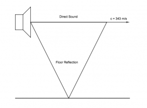
Sound velocity = 343 m / s
Direct Sound travels 1 / 343 = 0.0029 s = 2.9 ms (millisecond)
Floor Reflection path length = SQRT ( 1 + 4 ) = 2.236 m
Floor Reflection travels 2.236 / 343 = 0.0065 s = 6.5 ms
Reflection free window length = 6.5 – 2.9 = 3.6 ms
Such short windowing does not work at low frequencies. One cycle of 278 Hz takes 3.6 ms. If less than a cycle is contained within the measurement window, that frequency and all below it can not be calculated via FFT.
Near Field Measurements
To assist, we take near field measurements only a few mm away from the radiating surface. Here the ratio of direct to reflected sound SPL is high. Therefore hardly any influence of comb filtering.
Much more elaborate methods exist to calculate far field characteristics from near field measurements and simulation. But as a rapid estimation this formula works well to calculate half-space SPL at 1m from near field pressure data:
SPL (1m, HSP) = SPL (near field) + 20 * log ( 0.2821 * SQRT ( Sd) )
with Sd = diaphragm area in m2
Half space assumes that the loudspeaker radiates into a semi-sphere. This assumption is commonplace for such measurements and not completely absurd. Look at the wavelengths involved – for low frequencies our rooms are relatively small. And reflect low frequency energy similar to a half-space restriction of radiation.
You can measure high frequency data in the far field and splice near field low frequency data to the result to obtain a hybrid full-frequency response.
Data Discrepancy
Doing that, you will often recognise SPL abberations at the junction frequency. Because half space calculation does not include baffle diffraction effects. Nor does it consider diaphragm breakup. Sometimes reflex ports or other drivers leak into your near field measurement. And your far field measurement may have been closer than “far”.
Look at the picture on top of this blog: a horn system over 100 cm wide compared to a 24 cm wide near field monitor speaker. Transition of near field to far field is about 3-5 times away from the speaker dimension. Therefore 1 m distance is ok for the monitor, but NOT for the large horn system! Energy from various radiating surfaces arrives with different phase and will not sum up correctly at 1 m distance.
TestHifi uses a combination of sophisticated geometric averaging and adaptive windowing to achieve good results with short and easy measurements.
I hope to present some loudspeaker measurement examples next time.