Loudspeaker Measurements - Part 1

Part 1 – loudspeaker time domain and 1 m data

I would like to show some real nearfield and farfield measurements to underline my last blog about basic loudspeaker „frequency response“ measurements. As always, be aware I take shortcuts and do not cover more academic depths of nearfield radiation impedance etc. To focus on the basics, similar to how I measure speakers during crossover development.

Due to room influence measuring loudspeaker (LS) SPL versa frequency is a complex task, involving different LS and microphone („Mik“) positions. In order to cover the whole range from 20 Hz to 20 kHz in a meaningful way.

I start with presenting measured data taken with a time-windowing PC based system (Liberty Praxis). It produces logarithmic sweeps, and transforms the Mik output into impulse response, step response and frequency response. There are many other systems that perform similar tasks, like MLSSA, CLIO, ARTA and so on.

Usually, loudspeakers are specified with data related to 1 m distance

So what do we expect from measuring a stand-mounted 2-way LS, with it’s tweeter 126 cm above the floor? With the radiating surfaces covering 38 cm vertically and 14 cm horizontally? In a relatively large room of 240 m3?

Similar to the typical audiophile LS placement, the first and most unavoidable room reflexion comes from the floor. The speaker has 2 * 5 inch woofers, about 1 m above the floor. At 1 m distance, the reflexion will arrive at 1 m Mik height after travelling 2.24 m, which takes about 6.5 ms. Direct sound will travel 1 m and arrive after 2.9 ms.

Let us look at the impulse response at 1 m distance :

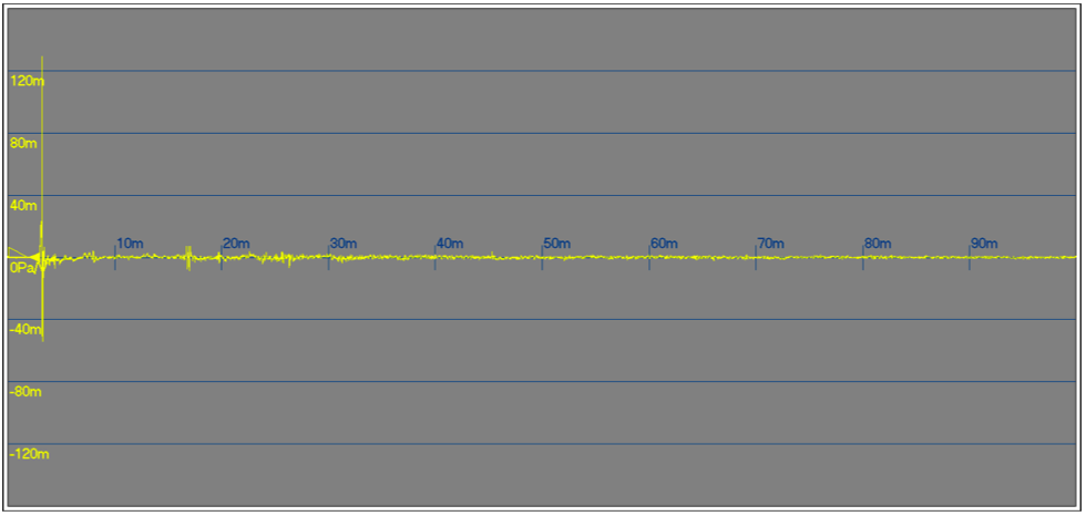
I choose a basic time window of 100 ms. Long enough for 10 Hz FFT resolution.
We find the initial impulse response at around 3 ms, followed by many smaller reflexions.
For a closer inspection of the first reflexions, we zoom into the first 10 ms of response :

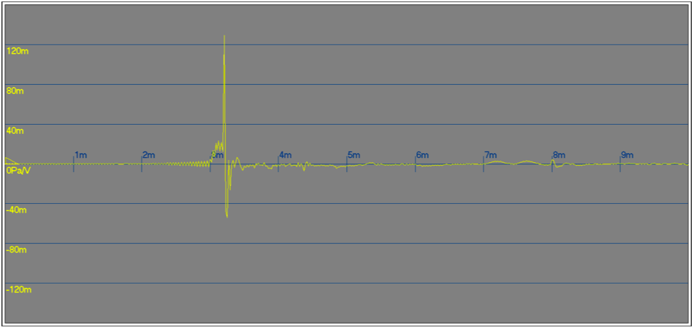
Due to a somewhat higher Mik-position the floor reflexion arrives between 6.9 – 8.2 ms.
It starts with the lower woofer (closest to the floor), and ends with the tweeter contribution.
Note some ringing in front of the real impulse due to digital artifacts.

Step response

Sometimes reflexions are easier to identify from the step-response, shown for comparison:

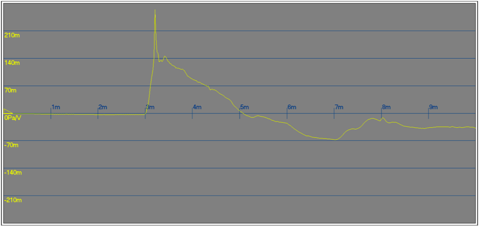
Why are the floor reflexions of both woofers and the tweeter separated in time between 7 – 8 ms, but not the direct sound?
Most loudspeakers disperse time, but these speakers are time-coherent designs. Most other speakers will produce direct sound impulse and step responses separated in time similar to their reflexions shown in my measurements. Look for example into stereophile (.com) speaker reviews to find more common step response characteristics.
That’s what you should measure with conventional multiway-loudspeaker. Sorry, but I don’t have such any more …
The floor reflexion is time-dispersed because the lower woofer is closer to the floor than the upper woofer and the tweeter (sitting on top).

Choosing a time window

The nice feature of a time domain based measuring system is the capability to separate reflexions from direct sound. To find out what „really“ comes from the speaker.
Let us now choose a short time window around the direct sound impulse response to ignore room contribution:

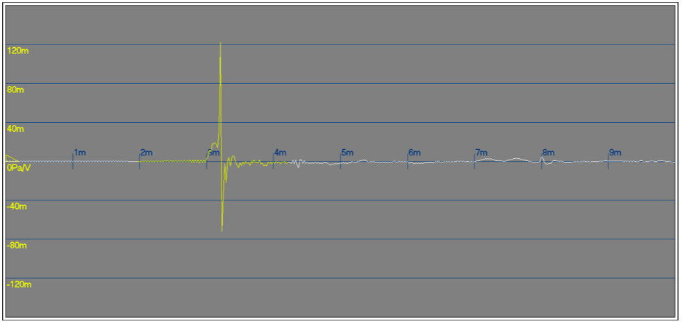
The yellow part is what we are going to transform into frequency domain via FFT. I choose a short 2 ms window to show the effect of short windows. This is a little too short for perfect FFT, due to windowing effects. The time window does not start and stop like a cutout, but has a more gentle filtering characteristic. Actually, you choose from many windows to use the best compromise between time leakage versa frequency domain precision. But let us inspect the result of the FFT.

SPL over frequency, 1 m distance

I will plot the 2 ms versa the full 100 ms window FFT.

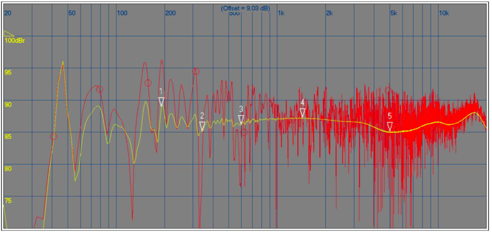
Please find the frequency scale on top (logarithmic, like our ear), and decibel at left (detto).
The strong room influence within 100 ms can easily be seen on the red trace. The smooth yellow curve shows the direct sound, at least for high frequencies. Of course, a 2 ms window is too short for low frequencies (LF)! Therefore, I use a flexible window that gets longer for LF, otherwise the curve would end at 500 Hz.
This is the reason why both curves get more similar at LF. And why the „2ms“ curve contains the same LF room effects like the „100ms“.

I recommend at least 3-4 ms window length if possible. These speakers have 88-89 dB sensitivity at 1 m / 2.83 V (as shown). Some of that energy gets lost due to the short „anechoic“ window. Forgive me for being lazy today, not placing the speaker on higher stands!

To be continued with other distances and the nearfield next time.