Fast Fourier Transformation
Today, Fast Fourier Transformation (FFT) based analyzer software is cheap or available for free. One such very nice and free program is REW (Room EQ Analyzer). It can do much more than analyze room acoustics, though I have little experience with that yet. Still … why not?
In one of my blogs I showed (a bit ridiculous, curious shot into the blue) measurements of „digital transports“.
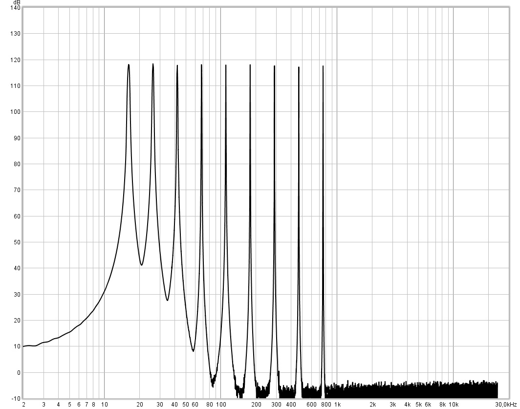
The top picture presents the spectrum of 9 test-tones, created digitally at 48 kHz with 16 bit resolution.
That signal’s wave-file was read by one PC, and in digital form (it was never converted to analog) sent through various components to another PC that runs the REW Software.
The question :
If the 9 sinusoidal test tones are perfect, why do the lower frequency (LF) tones show a widened spectrum at their base compared to higher frequency (HF) ones? A perfect sine should just be a vertical line …
Here’s for a simplified overview of basic FFT parameters:
Signal synthesis :
Look at the Fourier Transformation as a backwards analysis of a Fourier series (see https://en.wikipedia.org/wiki/Fourier_series). Imagine a Fourier series to be a way of assembling a periodic signal (to test our equipment) from several harmonic sinus components. These components can have different amplitudes and phase shift.
Digital signals :
Since we are in the digital domain, our signals are time-discrete digital samples instead of continuous waveforms. Therefore, we use a DFT (discrete Fourier transformation).
The FFT is a version of the DFT that is very efficient to compute. One characteristic of the FFT is that the number of samples analyzed is always a potency of 2 (2, 4, 8, 16, etc).
FFT size :
The FFT size is the number of samples analyzed. Let’s assume it to be 2^10 = 1024 samples. If our sampling frequency would be 40 times higher, that would be 40.960 Hz. Our FFT size would contain 1/40 of a second of the signal.
Frequency resolution :
Another characteristic of the FFT is that for an input size of 1024 samples it outputs 1024 different frequencies. The cycle of the lowest frequency analyzed can be no lower than the length of the FFT interval. For our example of 1/40 second that would be 40 Hz. All other frequencies are multiples of that.
Imagine a discrete spectrum like 40, 80, 120, 160 Hz, … frequency „bins“ that represent the content of our signal. Frequencies between those, such as 60 Hz, are represented by increased amplitudes at 40 and 80 Hz.
For look for lower frequencies and better resolution, we can either reduce the sampling frequency or increase the FFT size.
Windowing :
Our FFT size determines a number of samples which are cut out of the signal. At the beginning and end of that time „window“ through which we look at the signal, the signal will most often have a certain non-zero level.
Looking at the FFT block separated from the rest of the signal, at the beginning and end we have transients from zero the the respective start and endpoint sample levels. These transients „create“ frequencies that are not part of the original signal.
To avoid such misinterpretation in our FFT, we use a „window function“ to smoothly fade-in and out of the FFT block.
There is a trade-off between very smooth windowing and frequency resolution. A very smooth window will need more time to settle than a simple rectangular „cut- in and out“. But produces less artifacts.
In our example, the period of the lowest „visible“ frequency of 40 Hz equals FFT length at 1/40 second. Therefore, it’s whole cycle will be influenced by the window function, reducing the amplitude. Periodic signal components of higher frequency are less sensitive. Most of their cycles remain unchanged by the window function.
To sum it up :
We may choose to either evaluate sudden amplitude changes of HF signals with short FFT intervals OR look for lower frequency content within long FFT intervals. To aquire a „sharp picture“ of the frequency content we need a smooth time window, which again reduces the effective LF resolution.
The answer to above question :
To achieve the same resolution at all FFT frequencies we would need to apply a variable time window. Such „constant Q“ windowing contains the same number of cycles at all frequencies. In other words, it gets longer from HF to LF.
The other reason for the seemingly lower LF resolution of above plot is the logarithmic scale of the frequency axis. While the FFT delivers a linear frequency distribution, a certain length of the left-end frequency axis contains less frequency „bins“ than at the right (HF) end. Therefore, the picture looks sharper at the HF end.