
Listening Position Frequency Response
 Text to speech – Listening Position Frequency Response
Does measuring amplitude versa frequency (frequency response) at the listening position make sense?
I wrote about measuring at the listening position before, and covered room influence etc in other blog entries.
Today I would like to present some practical measurements to see if they represent what we can hear at the chosen listening position (LP).
Modal coupling
Let us start with measuring the same loudspeaker (LS) from the same listening position, placed at two slightly different locations:
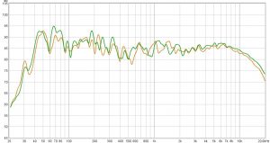
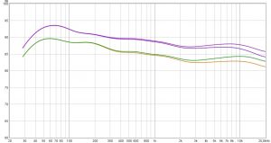
The top picture shows the response, measured with Room EQ Wizard (free for various platforms) and a cheap USB mic (UMIK-1 from miniDSP).
The room is about 10 m long, 4.5 – 5.5 m wide with a cathedral ceiling 3.5 – 4.5 m high.
LS are placed near to half length, where a room mode close to 30 Hz has a pressure maximum.
The chosen LP compensates this, set at about 1/4 length, where the same mode has very little pressure.
The light brown curve shows LS close to half length, green about 80 cm closer to the listening position.
Overall SPL around 30 Hz is low because of the chosen LP.
Moving forward takes the LS out of the maximum pressure zone, the glitch around 30 Hz in the response gets smoother. I could now move LP back to enjoy a stronger low end (not shown).
Besides LF details response curves like these are hard to read, due to strong high frequency (HF) interference with room reflexions.
Smoothing
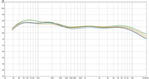
If we still want to see details in the response like resonances etc, we can smooth the curves just a little bit. Show below is the effect of 1/12 oct smoothing applied to the same curves as shown above. HF is now „readable“.
LP smoothed 1/12 oct
The LS uses dual woofers, on above the other. Due to their different floor distance this reflexion produces two notches around 500 and 800 Hz. Both are small in amplitude. The upper woofer is ex-Yamaha NS40, and the owner wanted to keep some „NS10 detail“ in the presence range. Therefore, I left some elevation in the 1-2 kHz region. The HF end shows SPL difference due to the green position moved towards the mic.
Overall, 1/12 oct smoothing shows both LF detail and readable HF, I recommend this as universal format with LP measurements.
Stronger smoothing
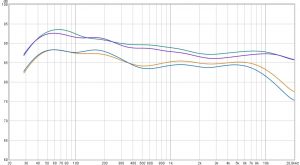
If we want to judge the LF / MF / HF balance of reproduction, we can apply 1 octave wide smoothing to the same data.
Below the response curves of both left and right LS:
LP octave wide smoothing
We can clearly see the relation of all 4 curves, generated by a pair of LS at similar room positions. Warm midrange and slightly pronounced presence may be expected. HF rollof is typical for larger dome diaphragms (1.2 inch used). Measured on axis without room influence it would be flat. Raising „bündelung“ with frequency radiates less HF energy into the room.
Loudspeaker comparisons
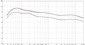
How about a comparison of two very different LS? Below, see the LS as discussed above compared to Betahorns. I’m currently working on the Beta’s, they are time-coherent now and sound much more relaxed than before. New cabinets, new drivers, new crossover – new loudspeaker within the same exterior shape.
Beta vs 10/8/1 inch
The upper curves show the Beta in it’s current status, the lower show the LS we had before. The new Beta LF geometry integrates the floor contribution in a way that avoids destructive interference – as can be seen in a flatter reponse around 400 Hz.
Both left and right (blue curves) LS shown – and here we can see a clear pattern that both speakers share:
The blue curves show a stronger low end of the midrange, the right position enhances the region around 180 Hz.
The LS themselves are obviously different, we can see why the Beta sound so relaxed: very linear decrease of SPL throughout the midrange towards HF. Slight depression of „detail range“ around 2.7 kHz. More SPL above 8 kHz.
Interestingly the Beta sounds less „hot“ at HF than the other LS, and still more detailed. Advantage of the horn, less room influence that masks the sound. The overall sound of the Beta now approaches that of the system I described in my very subjective Phase and Time 2 blog. Huge, open and relaxed, a joy to listen to, but not quite real (whatever this is). Which the measurement does show. Finally I will make it a little more forward … only a little bit 🙂
Can tiny details be measured at the LP?
While the overall Betahorn update is done, I still work on small details to fine-tune the response.
Eg there is an acoustic lens in front of the woofer, that influences the lower midrange.
Since the sound was a little too warm in the midrange, I modified it. The same could be done with a crossover mod, but I prefer minimal parts count (one coil instead of 12 parts with the previous generation. Less is more).
The effect of this modification is shown below, again with 1-octave wide smoothing, left and right LS:
Beta LF lens mod
Let us just say it works! Looking close, we can even see the influence in the detail range. The modified lens has stronger low-pass character which smoothes the 2.7 kHz region a bit. Listening proofs: midrange is done.
Influence on tube amplification
I finally connected the Beta prototypes to an EL84 PP tube amplifier. This amplifier has higher source impedance than usual transistor amps. Which „distorts“ the frequency response if the LS impedance varies with frequency.
In our case, the impedance raises above 300 Hz, which I correct inside the crossover. That circuit can be disconnected (remember, less is more), with it’s effect shown below:
Beta Z-Korr Influence
I shifted the left LS responses +3 dB for better readout. Both channels show more HF SPL due to higher impedance here, with disconnected impedance correction. A nice way to try out how a more „forward“ Beta may sound.
What all these SPL (sound pressure level) versa frequency measurements do not show:
Changing from transistor to tube amplification changes the sound a lot. With the tube amp producing much more realistic sound. Strings from an orchestra sound like strings, less like modulated noise. New details emerge, and lyrics are much easier understood. With or without impedance correction.
Conclusion
We can measure small changes to our system with simple means. Changes to the LS, even if buried in the room response. And changes to the room influence, like a new LS position. This helps to judge if the change influences the right portion of the audio spectrum as desired. But not everything that influences the sound quality is represented in frequency response measurements.